Other Risk Measures

There are other ways to measure risk besides standard deviation. Two other common risk measures are semi-deviation and Value-at-Risk (written as VaR).

Semi-Deviation

If you were given two stocks, one that continued to increase by 10% every day, and one that decreased by 10% every day, would you intuitively think that one stock was more risky than the other? Standard deviation measures of risk would give these two stocks the same level of risk, but you might think that investors are more worried about down-side risk (when stocks decline), rather than upside risk. The motivation for semi-deviation measure of risk is to measure downside risk specifically, rather than any kind of volatility.

Semi-deviation is calculated in a similar way as standard deviation, except it only includes observations that are less than the mean.

SemiDeviation = \sum_{t=1}^{n}(\mu - r_i)^2 \times I_{r_i<\mu}
where I_{r_i < \mu} equals 1 when r_i < \mu , and 0 otherwise.

Value-at-Risk (VaR)

VaR, or value-at-risk is a portfolio risk measure. Risk managers at investment firms and investment banks calculate VaR to estimate how much money a portfolio manager’s fund may potentially lose over a certain time period. Corporations also estimate their own VaR to decide how much cash they should hold to avoid bankruptcy during a worst case scenario.

VaR is defined as the maximum dollar amount expected to be lost over a given time horizon at a predefined confidence level. For example, if the 95% one month VaR is $1 million, there is 95% confidence that the portfolio will not lose more than $1 million next month. Another way to describe the VaR is that there is a 5% chance of losing $1 million or more next month. The methods for calculating VaR are beyond the scope of this lesson, but if you ever become a risk manager, or ever work with a risk manager, you’ll probably see Value-at-Risk quite a bit.

For a visual representation of VaR, we can look at a data distribution that represents the rate of return of a stock. If we color in the area in the left tail that represents 5% of the distribution, the rate of return represented by that point on the horizontal axis is the rate of return that may occur in the 5% worst case scenario. To convert that to a VaR, we multiply that rate of return by the amount of capital that is exposed to risk. For a portfolio, it would be the amount of dollars invested in that particular stock.

As an example, let’s say we invested $10 million in a stock. We estimate the mean and standard deviation of the stock’s returns and model it with a distribution function (it might be a normal distribution, but there are other models). Then we find the rate of return that defines 5% of the distribution to its left, in the left tail. Let’s say that rate of return is -20%. We multiply that rate of return by the amount that we’re exposed to, which is -0.20 \times \$10 million = -\$2 million . So the VaR on any given day is $2 million. In other words, we may plan some hedging strategies or hold enough cash to help us handle the possibility of losing $2 million on stock A on any given day.
For more detail, and an image of the distribution, check out Wikipedia’s page on Value-at-Risk

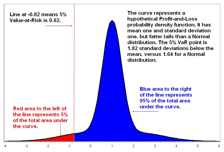
This diagram of VaR is from Wikipedia's page on Value at Risk